It’s the million-dollar data science question: How much data do I need to produce a high-quality marketing attribution model, one that can accurately determine the contribution of different marketing channels to a conversion?
This question has been asked of data scientists countless times, and the answer has always contained the same two words: It depends.
But we can do a little better than that. While there’s no answer truly set in stone, we can study our existing models and begin to build up a working understanding of what has worked in the past. This understanding will grow as more models are built and more edge cases are discovered.
How to Quantify the Quality of an Attribution Model
Let’s start by identifying a metric that can be used to quantify the quality of a model. The coefficient of determination, commonly referred to as “R squared,” is frequently used for just this purpose.
The R squared metric compares how well your model describes the data compared to a model that guesses the average value no matter the input data. If your model provides more accurate predictions than the average value, you will see an R squared close to 1.
The closer your model gets to simply predicting the average value, the closer your R squared will get to 0. In the unfortunate case that your model is somehow worse than just guessing the average value, you will see your R squared drop below 0.
Testing Your Attribution Model
Now that we know how we intend to judge our models, let’s start experimenting. It’s common practice in data science to randomly choose data to withhold from the training process. This means that we train the model using only a portion of the data, say 80 percent, and keep the remaining 20 percent unseen. The unseen data can then be used to test how well the model performs on new inputs.
We don’t want a model that memorizes training data. We want a model that understands the trends in the training data and can extrapolate out to data it’s never seen. For this reason, we will measure our R squared using only the testing data.
But this introduces a problem: The data points in the test set are chosen randomly. This means that our R squared metric will depend on which points are chosen at random. How are we supposed to compare models fit on different datasets if our comparison metric depends on a random choice? Does one model have a higher R squared value than the other because it’s a better model? Or is it because random chance provided a nicer testing set to one model than the other?
The answer is actually quite simple. We run through the process multiple times. This allows us to see how much our R squared changes as we randomly shuffle points between our training and testing sets.
What We Can Learn About Our Models
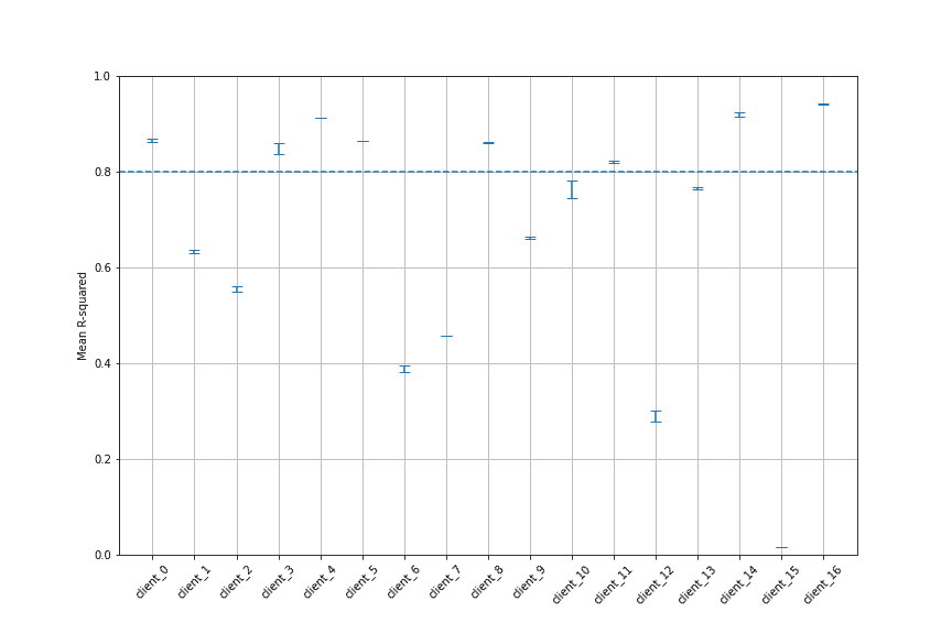
After we have applied our testing strategy to multiple datasets, we can visualize the results across the datasets and start making choices about what we think is a good or bad model. This is where we have to be subjective and define a criteria based on our understanding of the problem and our goals for the model. As we build more models and our understanding grows, this criteria will grow and adapt as well.
For this example, we defined two criteria as a starting point for determining what is a good model:
- We want the lowest trial R squared value to be greater than 0.8.
- We want the variation in R squared between trials to be small.

We wanted to see how the amount of data available might impact the quality of the model. So we investigated the effect of the longest channel length (the channel with the most data), the shortest channel length (the channel with the least data) and the number of channels in the model.
From our study, we see that all datasets containing greater than three years of historical data produce good models. In contrast, we were unable to produce good models for datasets with less than 1.25 years of historical data. The range in between 1.25 and 3 years of data depends more heavily on the contents of the dataset and requires further study.
(That’s not to say that you can’t build good models for shorter datasets — this is actually something we can help our clients with.)
The amount of data in the shortest channel does not appear to have an effect on the overall quality of the model. This may have a larger effect on models attempting to make predictions.
We found that most attribution models are driven heavily by one or two channels with much smaller contributions from any additional channels. This is even more true in the datasets we identified as providing good models, which always had four or more channels present. In these cases, typically one and sometimes two channels would provide the most impact while the remaining channels were much less impactful.
With Attribution Modeling, Insight Builds on Insight
While this analysis doesn’t provide a hard and fast rule for what makes a good model, it shows how we can investigate our existing datasets to gain insight into what has worked in the past. We can use these insights to advise our decisions in the future.
Every dataset is different, and there’s no guarantee that a given model will meet expectations on a given dataset, but the insights we gain empower us to make informed decisions, allowing us to improve efficiency and increase value from marketing investment.
Multi-Channel Attribution Made Simple
Alight’s end-to-end analytics solutions feature multi-channel attribution models, built right into Power BI or Tableau, to help you reduce the time and cost to generate a conversion. Schedule a free solution consultation with our team!

